Genetic drift

Genetic drift is the violation of the 5th assumption of HWE in Mendelian inheritance: gametes are drawn infinitely and with replacement.

Effects of finite sampling

Finite sampling means there is random variation at each generation. In practice we still consider sampling is done with replacement.

For example, with a population size of 10:

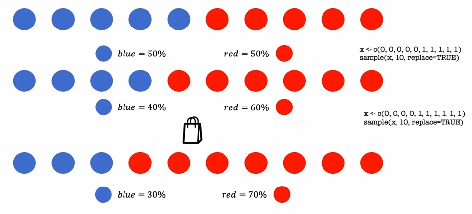
Binomial distribution

This random change can be modeled probabilistically with binomial distributions.

$$P(\text{i alleles of B})=\left(\genfrac{}{}{0ex}{}{2N}{i}\right)p^i{q}^{2N-i}$$

Wright-Fischer model

Simplest model of genetic drift.

Suppose N diploid parents producing an infinite number of gametes that pair randomly. Individuals are hermaphroditic (have a $\frac{1}{N}$ probability of reproducing with themselves).

The transition matrix between states $j$ and $i$ has the coefficients:

$$x_{ij}=\left(\genfrac{}{}{0ex}{}{2N}{2N-i}\right)(1-\frac{j}{2N}{)}^{2N-i}(\frac{j}{2N}{)}^i$$

$x_{ij}$ is the probability of being in state $i$ at time $t+1$ after being in state $j$ at time $t$.

For example, if $2N=4$:

	0	1	2	3	4
0	1	0.316	0.25	0.004
1		0.422	0.25	0.047
2		0.211	0.375	0.211
3		0.047	0.25	0.422
4		0.004	0.25	0.316	1

Columns with a $1$ are called absorbing states because they lead to loss or fixation.

If we start with a number of alleles $i$, we have the vector $Y_0$ with a single $1$ at index $i$. Then for any time $t$, the probability distribution will be $Y_t=X^t{Y}_0$.

For example, if $i=2$:

	1	2	…	$\infty$
0	0	0.063		0.5
1	0	0.25		0
2	1	0.375		0
3	0	0.25		0
4	0	0.063		0.5

Genetic drift leads to loss or fixation of an allele. The probability of fixation of an allele is its initial frequency $p_0$ in the population, and the probability of loss is $1-p_0$. For a new mutation, it is $\frac{1}{2N}$.

The average frequency of an allele is expected to stay the same. The variance is based on that of he binomial distribution.

Heterozygosity ($H_t$) decreases with time and population size ($N$):

$$H_t=2\sum _{j=0}^{2N}(1-\frac{j}{2N})\frac{j}{2N}{y}_{jt}$$

The time to fixation is:

$$T(p)=\frac{1}{p}\sum _{t=1}^{\infty }t(y_{2N,t}-y_{2N,t-1})$$

From the Diffusion approximation:

$$T(p)=-\frac{4N(1-p)\ln (1-p)}{p}$$

As $p$ becomes small:

$$T(p)=4N$$

The age of an allele can be estimated from its frequency:

$$t\approx -\frac{4Np\ln (p)}{1-p}$$

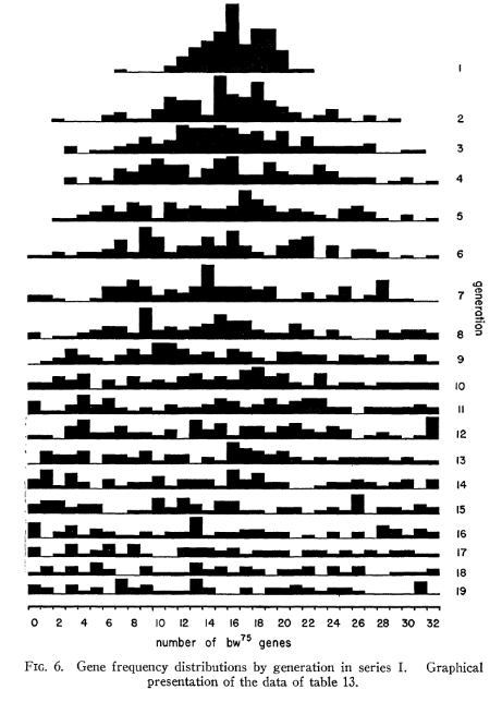
Buri (1956)¹ examined genetic drift in fruit fly populations for the $b{w}^{75}$ allele. He verified the predictions of the Wright-Fischer model.

Inbreeding

Inbreeding means individuals share a common ancestor.

F-statistics quantify drift and inbreeding. F is a measure of identity by descent (IBD).

$$F_t=\frac{1}{2N}+(1-\frac{1}{2N})F_{t-1}$$ $$1-F_t=1-[\frac{1}{2N}-(1+\frac{1}{2N})F_{t-1}]$$ $$1-F_t=(1-F_{t-1})(1-\frac{1}{2N})$$ $$1-F_t=(1-F_0)(1-\frac{1}{2N}{)}^t$$

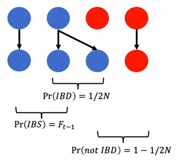
As $t$ gets large, $F_t$ tend s to $1$, meaning everyone is IBD.

Coalescence

The reverse of F-stats: going back in time to see when everyone was related.

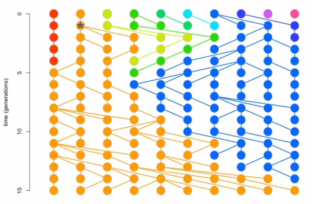
For example, there are 10 lineages at $t=0$. By $t=15$, only 1 is left.

Forxard in time, the orange lineage has been fixed. Backward in time, the orange lineage coalesces into a single ancestor at $t=2$.

For each generation, the probability of coalescence is

$$P(\lambda )=\frac{1}{2N}$$

For any number of lineages $i$, the average time is

$$T(\lambda )=\frac{4N}{i(i-1)}$$

The average time for two lineages to coalesce is

$$T(\lambda )=\frac{4N}{2(2-1)}=2N$$

If $i$ is large, most coalescence occurs rapidly. On average, half of the waiting time for coalescence is in the last two lineages ($2N$).

Effective population size

The $N$ in those equations is the effective population size. It does not match the actual number of individuals. Drift can happen at a rate corresponding to a way smaller or larger population size.

The effective population size $N_e$ is the rate of drift in an idealized Wright-Fischer population.

$$N_e=\frac{p(1-p)}{2\text{var}(\Delta p)}$$

$N_e$ can be different from $N$ because of

• Breeding structure: if only a few males reproduce, drift happens faster
• Population size fluctuations: $N_e$ is the harmonic mean of population size over time, which is sensitive to small values
• Population structure: if there are small isolated populations, drift is slower because variants are slowly transmitted between groups
• Natural selection

---

From Zach B. Hancock, Genetic Drift | The Causes of Evolution | Ep. 5

Footnotes

1. Buri (1956), Gene frequency in small populations of mutant drosophila ↩