Discovering a fractal

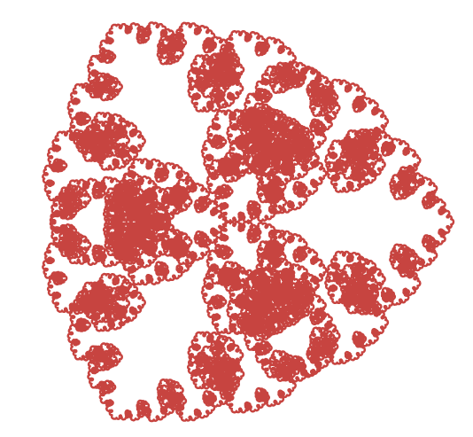
So, I discovered a fractal. Multiple fractals actually. These beautiful figures were hidden behind one of math’s most infamous monsters. We will explore mathematical grounds that were once considered safe and tame, discover a monster that broke a generation of mathematicians, then build beautiful fractals from this monster, and finally explore some of their properties.

The Weierstrass function

Everything starts with the Weierstrass function. In order to understand what it is and why we care about it in the first place, let’s talk about continuity and differentiability.

We usually say a function is continuous when we can draw its line graph without lifting our pencil. In more rigorous terms, a function $f$ is continuous at the point $p$ if the limit of $f(x)$ as $x$ tends to $p$ is equal to $f(p)$. This neatly encapsulates the intuition we have of continuity. However notice that the exact definition only tells us about continuity at a single point. We say a function is continuous on a line segment if it continuous at all of its points. Similarly, a function is continuous on $\mathbb{R}$, the set of real numbers, if it is continuous at each and every real number.

On the other hand, we say a function is differentiable when it has a well-defined, finite slope. In more rigorous terms, a function $f$ is differentiable at the point $p$ when its growth rate converges.

$$f^{\prime }(p)=\underset{x\to p}{\lim }\frac{f(x)-f(p)}{x-p}$$

Notice once again that the definition only tells us about differentiability on a single point. Again, a function is differentiable on $\mathbb{R}$ when it is differentiable on all real numbers.

It is worth noting that differentiability implies continuity. A function can only be differentiable if it is already continuous. The converse is not necessarily true.

As a counter-example, we can look at the function $|x|$. It is continuous on $\mathbb{R}$. The left-hand part is differentiable and its derivative is -1, the right-hand part is differentiable and its derivative is 1. What happens at 0 is quite literally an edge case: the derivative can not exist, because the growth rate converges towards a different value depending on the side we compute it on.

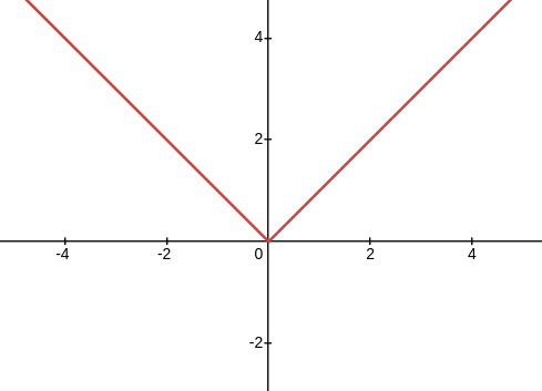
This example has a single non-differentiable point. And if you try to come up with your own counter-examples, you will likely end up with continuous functions with a few undifferentiable points. This begs the question: can a continuous function be not differentiable on a whole line segment, or even on all $\mathbb{R}$? Mathematicians who originally came up with counter-examples like ours thought that no, undifferentiability of continuous functions were localized to some points, that those points couldn’t be everywhere. However, they were proven wrong by the Weierstrass function.

What’s this function? It is defined as the sum of infinitely many cosines. The frequency of those cosines grows following $b^n$, and those cosines are weighted following $a^n$.

$$W(x)=\sum _{n=0}^{\infty }{a}^n\cos (b^n\pi x)$$

We add the condition that $ab>1$. This ensures that as $n$ grows, the frequency $b^n$ grows faster than the amplitude $a^n$ shrinks. If $ab<1$, the amplitudes would die off fast enough to tame the slopes, and the function could end up differentiable after all. The case where $ab=1$ is a limit case that depends on the specific value of $a$. The condition $ab>1$ is precisely what keeps the derivative from ever settling down.

You will often see this function with the specific values $a=\frac{1}{2}$ and $b=4$:

$$W(x)=\sum _{n=0}^{\infty }\frac{\cos (4^n\pi x)}{2^n}$$

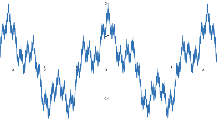
And this function is very special, it is continuous everywhere on $\mathbb{R}$, but differentiable nowhere. Now let’s explain why this is the case. Continuity and differentiability both behave nicely when building functions from other ones. A finite sum of continuous functions is continuous, and a finite sum of differentiable functions is differentiable. This is also true for products, and even for compositions. This allows us to easily prove many of the usual functions are neatly continuous and differentiable, like polynomials for instance. The subtle property that will play a crucial role is that this property is only automatic for finite sums. When we have an infinite sum like with the Weierstrass function, things get trickier.

Looking back at our function’s definition, we can look at the different sines it’s made up of to understand how the partial sums converge towards the whole function. We know the cosine function is bounded between -1 and 1. For the $a$ and $b$ values we took as an example, that means that every term’s absolute value is bounded by $\frac{1}{2^n}$.

$$W(x)-\sum _{k=0}^n\frac{\cos (4^k\pi x)}{2^k}=\sum _{k=n+1}^{\infty }\frac{\cos (4^k\pi x)}{2^k}$$ $$|W(x)-\sum _{k=0}^n\frac{\cos (4^k\pi x)}{2^k}|\le \sum _{k=n+1}^{\infty }|\frac{\cos (4^k\pi x)}{2^k}|$$

Therefore, the difference between the partial sums and the complete function is always uniformly bounded by the sum of $\frac{1}{2^k}$ for k going from $n+1$ to infinity.

$$|W(x)-\sum _{k=0}^n\frac{\cos (4^k\pi x)}{2^k}|\le \sum _{k=n+1}^{\infty }\frac{1}{2^k}$$

The sequence on the right converges towards 0, so this difference is a function whose bounds converge towards 0 as well.

$$|W(x)-\sum _{k=0}^n\frac{\cos (4^k\pi x)}{2^k}|\to 0$$

We call this uniform convergence. And it’s the most important hypothesis of the theorem that proves the Weierstrass function is continuous.

On the other hand, if we compute the derivatives of those sines, we notice that the $4^n$ inside is taken out. Their derivatives are equal to $-2^n\pi \sin (4^n\pi x)$.

$$\frac{d}{dx}\left(\frac{\cos (4^n\pi x)}{2^n}\right)=\frac{-4^n\pi \sin (4^n\pi x)}{2^n}=-2^n\pi \sin (4^n\pi x)$$

We can see the exponential factor $2^n$ making the terms blow up to infinity if we try computing the derivative. This is visible when we look at the graphs of those cosines: although they get smaller in amplitude, their frequencies grow even faster than their amplitudes do.

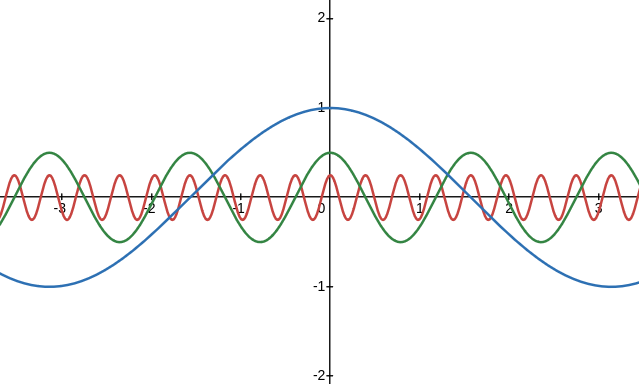
So obviously their slopes grow larger exponentially, and the sum diverges to infinity. In short: the frequencies grow faster than the amplitudes shrink, and that imbalance is exactly what makes the function nowhere differentiable.

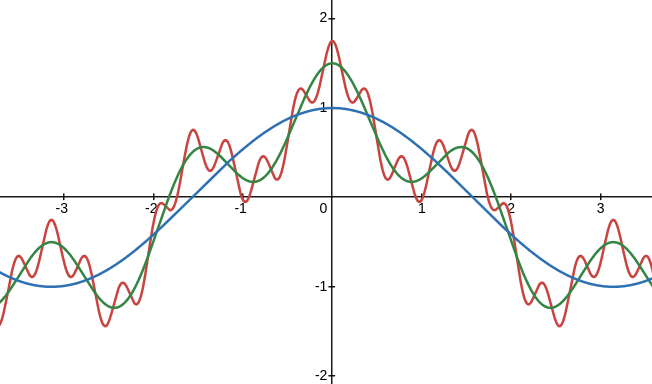
This tells us the partial sums’ derivatives diverge, but it doesn’t immediately prove the full function is nowhere differentiable, that requires a more careful argument about difference quotients that I’ll spare you here. The intuition is solid though: the frequencies grow faster than the amplitudes shrink, and that imbalance is exactly what makes the function nowhere differentiable.

And this explains why the Weierstrass function is continuous everywhere and differentiable nowhere. We can zoom to any point of its graph, and always see more details. It is impossible to even tell if the function is going up or down at any given point.

Building the fractal

So, we’ve seen the Weierstrass function is a sum of cosines, with different frequencies and different amplitudes. The trick is to treat the Weierstrass function as the real part of something larger.

To understand the trick, we need to talk about complex numbers for a moment. A complex number is just a pair of real numbers, a real part and an imaginary part, that we write as $a+bi$, where $i=\sqrt{-1}$​. We can think of complex numbers as points in a 2D plane, where the horizontal axis is the real part and the vertical axis is the imaginary part.

Now, what happens when we compute $e^{ix}$ for a real number $x$? There’s a remarkable theorem called Euler’s formula that tells us:

$$e^{ix}=\cos x+i\sin x$$

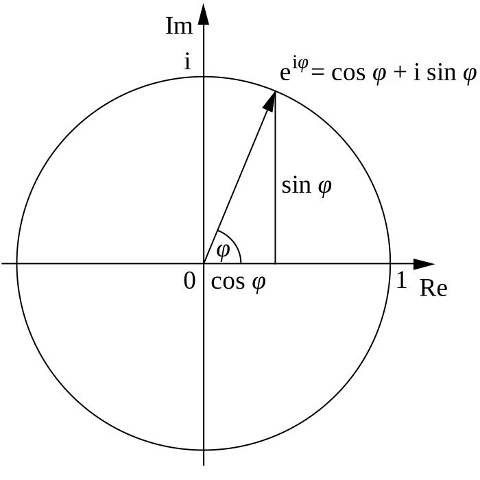
This is the most important formula tying together complex numbers and trigonometry. Sine and cosine are dual functions in some way, the exponential of a pure imaginary number decomposes into a real cosine and an imaginary sine. What this means geometrically is that as $x$ grows, the point $e^{ix}$ traces a circle of radius 1 in the complex plane. And since this is a linear equality, it can apply to sums of sines and cosines as well. For example:

$$e^{ix}+\frac{1}{2}{e}^{4ix}=\cos x+\frac{1}{2}\cos \left(4x\right)+i\sin x+i\frac{1}{2}\sin \left(4x\right)$$

Since $e^{ix}$ traces a circle in the complex plane, a sum like $e^{ix}+\frac{1}{2}{e}^{4ix}$ traces a more complex path: one circle riding on top of another. These nested rotating circles are called epicycles, and their combined tip traces a curve in the plane. The simplest epicycle is a boring circle, corresponding to the function $e^{ix}$. The epicycle corresponding to $e^{ix}+\frac{1}{2}{e}^{4ix}$ looks like this:

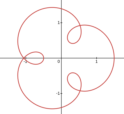
An interesting property of epicycles is their symmetry. When the epicycle is the sum of a real cosine and an imaginary sine, the figure is symmetrical with respect to the horizontal axis. Why? On one hand cos is symmetric, meaning that for any $x$, $\cos (-x)=\cos (x)$. On the other hand sin is antisymmetric, meaning that for any $x$, $\sin (-x)=-\sin (x)$. Therefore when tracing the figure the other way around, we simply trace the same figure with its vertical axis (determined by sines) flipped.

This is the bridge we need. Cosine, which appears in the Weierstrass function, is exactly the horizontal coordinate of this circular motion. So the Weierstrass function, a sum of cosines, is really just the horizontal shadow of something rotating in the complex plane. And if we stop projecting down to just the horizontal axis, and instead watch the full 2D motion, we get something richer. We can do the same with the Weierstrass function. We can see it as the real part of a complex function that we’ll call $\tilde{W}$:

$$\tilde{W}(x)=\sum _{n=0}^{\infty }{a}^n{e}^{i{b}^{n}2\pi x}$$

I chose to put $2\pi x$ rather than $\pi x$ in the exponential, because it makes the function 1-periodic ($\tilde{W}(x+1)=\tilde{W}(x)$) and therefore a bit nicer to manipulate.

We therefore have:

$$W(2x)=\text{Re}(\tilde{W}(x))$$

And by plotting this complex function with the parameters $a=\frac{1}{2}$ and $b=4$, we get our new fractal. I’ll name it quite naturally the Weierstrass fractal.

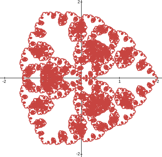
The function is impossible to truly represent because of its infinite sum. The representations used here use a partial sum with $n$ from $0$ to $7$.

Plugging other values for $b$ yields different figures. When $b$ is an integer, we get neat figures that seem to have $b-1$ axes of symmetry.

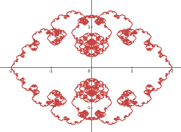
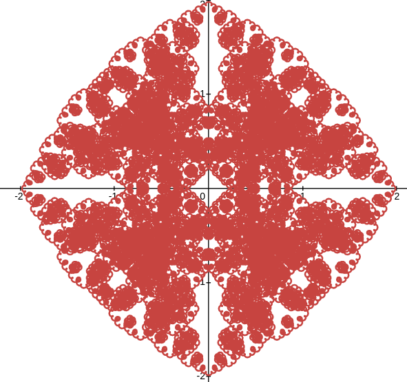
When $b$ isn’t an integer, we get very messy non-repeating figures that fill out the space.

And when $b$ is negative, we get even more fractals! Those look like stars with $1-b$ branches. for $b=-4$, it’s a 5-branched star.

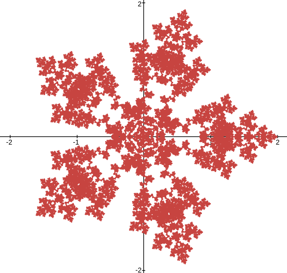
Changing $a$ only changes the size and thickness of the fractal.

Well, to be honest, during the writing of this video I found a blog post about epicycle fractals which also features this fractal. Here’s an animation from the post:

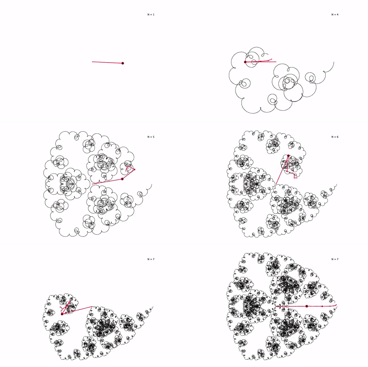
In order to make up for my utter lack of originality, I will go further and explore mathematical properties of this fractal.

Symmetries

The first property we can explore is its symmetry. We can see that when $b=4$, the fractal has radial symmetry with respect to 3 axes, and central symmetry with angle $\frac{2\pi }{3}$. In order to properly demonstrate this, we have to formalize it.

Having this symmetry means a point belongs to the line graph if and only if the same point rotated by $\frac{2\pi }{3}$ belongs to the line graph as well. In the complex numbers, we have a simple way of writing rotations: we multiply with unit complex numbers. The number $1$ represents as rotation of 0 radians. Multiplying by $i$ represents a rotation of $\frac{\pi }{2}$ radians, or one quarter of a circle. Multiplying by $-1$ is a rotation of $\pi$ radians or half a circle. And in our case, a rotation of a third of a circle corresponds to multiplying by $e^{\frac{i2\pi }{3}}$, often noted $j$. This number has some useful properties: $j^3=1$, $j^4=j$, etc.

So we have to show that if a point $p$ exists in the line graph, meaning there is a number $x$ such that $\tilde{W}(x)=p$ if and only if there is a number $x^{\prime }$ such that $\tilde{W}(x^{\prime })=jp$. Since the complex Weierstrass function is a periodic function, we can expect that shifting the function by a third of its period yields the same points rotated by a factor of $j$:

$$\tilde{W}(x+\frac{1}{3})=j\tilde{W}(x)$$

Let’s prove this. For any $x$:

$$\tilde{W}(x+\frac{1}{3})=\sum _{n=0}^{\infty }\frac{e^{i{4}^{n}2\pi (x+\frac{1}{3})}}{2^n}$$

Factoring out the additional term:

$$\tilde{W}(x+\frac{1}{3})=\sum _{n=0}^{\infty }\frac{e^{i{4}^{n}2\pi x+i\frac{4^{n}2\pi }{3}}}{2^n}$$

We can use the properties of the exponential to take out that term:

$$\tilde{W}(x+\frac{1}{3})=\sum _{n=0}^{\infty }\frac{e^{i{4}^{n}2\pi x}{e}^{i\frac{4^{n}2\pi }{3}}}{2^n}$$

That multiplicative term looks suspiciously like $j$. By taking out the $4^n$ exponential, it’s even clearer:

$$e^{i\frac{4^{n}2\pi }{3}}=(e^{i\frac{2\pi }{3}}{)}^{4^n}$$

Thus:

$$e^{i\frac{4^{n}2\pi }{3}}=j^{4^n}$$

Remember when we said that $j^4=j$? Well it also means that ${j^4}^2=j^4=j$. More generally, $j^{4^n}=j^{4^n\mathrm{mod}3}$. Since $4=1\mathrm{mod}3$, we get $4^n=1\mathrm{mod}3$ for all $n\ge 0$. Thus $j^{4^n}=j^1=j$, and:

$$e^{i\frac{4^{n}2\pi }{3}}=j$$

Going back to our equations on the complex Weierstrass function:

$$\tilde{W}(x+\frac{1}{3})=\sum _{n=0}^{\infty }\frac{j{e}^{i{4}^{n}2\pi x}}{2^n}$$

Thus:

$$\tilde{W}(x+\frac{1}{3})=j\sum _{n=0}^{\infty }\frac{e^{i{4}^{n}2\pi x}}{2^n}$$

Meaning we finally have:

$$\tilde{W}(x+\frac{1}{3})=j\tilde{W}(x)$$

Therefore proving central symmetry.

The axial symmetry follows from two facts together:

• First, $\tilde{W}$ is an epicycle built from cosines (real part) and sines (imaginary part). Since cosine is even and sine is odd, the figure is symmetric with respect to the real axis, aka the horizontal axis.
• Second, we just proved the figure has 3-fold rotational symmetry. A figure that has both one axis of symmetry and n-fold rotational symmetry necessarily has n axes of symmetry total, each separated by an angle of $\frac{\pi }{n}$​. Applying this with $n=3$: the horizontal axis of symmetry, combined with rotational symmetry of order 3, generates two further axes of symmetry at angles $\frac{\pi }{3}$​ and $\frac{2\pi }{3}$​ from it. This yields the 3 axes visible in the figure.

The same reasoning can be applied for other values of $b$. For $b=5$, the figure has 4-fold central rotational symmetry and 4 axes of symmetry. In fact, the fractal has $b-1$ fold symmetry, for all integers $b$ greater or equal to 2, and $1-b$ fold symmetry for all integers $b$ less than or equal to -1.

Dimension

An interesting property of fractals is that they have a dimension that’s typically not an integer. Lines have dimension 1, surfaces have dimension 2, volumes have dimension 3. But fractals sitting in a 2D plane typically have a dimension of somewhere between 1 and 2, and fractals sitting in a 3D volume between 2 and 3.

One approach to calculating a fractal’s dimension is called box counting, sometimes called Minkowski–Bouligand dimension.

The core of the idea is to place the figure in a grid of squares of a given size, and see how many squares are needed to cover the figure As the size of the squares scales down, the number of squares required scales up. And the relationship between those two scaling factors gives the dimension. The advantage of this approach is that it works computationally, and doesn’t require self-similarity.

When writing $d$ the fractal’s dimension, $ϵ$ the side length and $N(ϵ)$ the associated number of boxes required to cover the set, the scaling relationship is:

$$N(ϵ)=(\frac{1}{ϵ}{)}^d$$

Using logarithms, we get:

$$\log (N(ϵ))=d\log (\frac{1}{ϵ})$$

Thus:

$$d=\frac{\log (N(ϵ))}{\log (\frac{1}{ϵ})}$$

I wrote a Python script to compute the box-counting dimension. It calculates an approximation of the function with a fixed number of points, computes the number of squares $N(ϵ)$ for 10 values of logarithmically spaced $ϵ$, then runs a linear regression on the logarithms to get the value of $d$ from the slope.

The script also shows the graph, which allows to visually confirm enough points were computed with enough precision. If the points stop following the same trend for small sizes $ϵ$, it means the squares are getting to small and we need a more precise approximation.

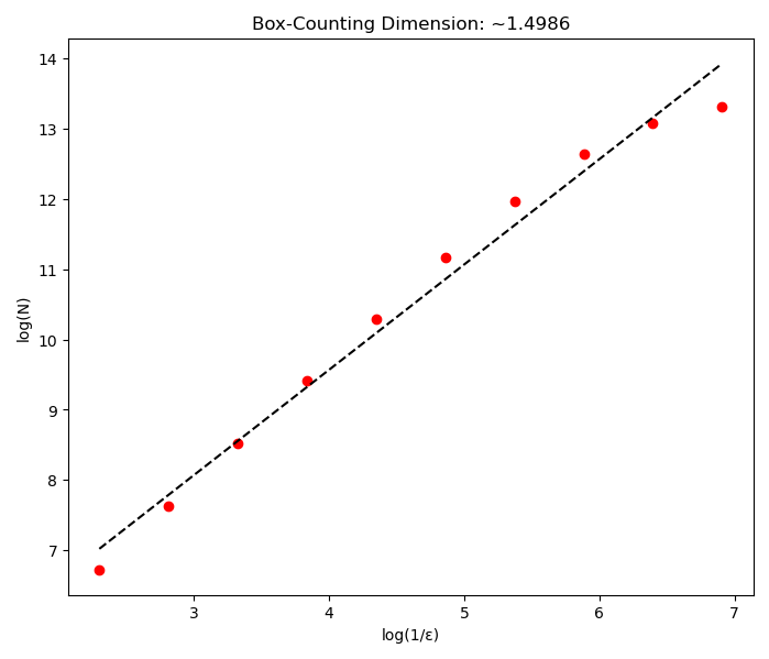
To make sure the result is reasonably correct, we simply have to increase the number of data points until the points are well-aligned.

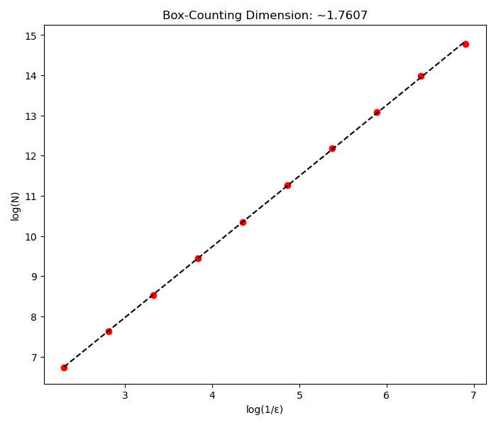
For $b=4$, the computed box-counting dimension is 1.7503. We can run the script for multiple values of $b$, which gives:

b	dimension
-4	1.7623
-3	1.5521
-2	1.0762
2	1.0936
3	1.5485
4	1.7503
5	1.8425

A few things are worth noticing:

• First, $b=2$ and $b=-2$ both give dimensions close to 1: those fractals are nearly one-dimensional curves, barely filling the plane at all. this is the edge case when $ab=1$. As $\mid b\mid$ grows, the dimension climbs towards 2, meaning the fractal fills more and more of the plane.
• Second, positive and negative values of $b$ with the same absolute value give very similar dimensions. The star shape and the triangle shape are geometrically different, but they fill space at roughly the same rate.

There is a second way of considering dimension: the Hausdorff dimension. It is more formal, but also harder. The figure does show self-similarity, it contains approximate smaller copies of itself at varying scales. However I haven’t succeeded in finding patterns consistent enough so far.

The curve of the original Weierstrass function does have a Hausdorff dimension of $2+\frac{\log a}{\log b}$, but this doesn’t automatically translate into the epicycle, and isn’t consistent with the box-counting dimensions we just computed. This isn’t really surprising, the Weierstrass function’s graph and our fractal are different in nature. Our fractal occupies the plane and intersects itself, providing a richer and more complex structure.

I haven’t found a closed formula for the Hausdorff dimension. This remains an open question worth exploring.

Conclusion

It’s revealing of what happens in math: we discover monsters that question our previous assumptions and breaks our intuitions. Then we tame those monsters, explore their behavior, and sometimes find beauty in what they have to offer. And this is a continuous process that always leaves mystery on the table, as shown by the Hausdorff dimension we talked about.